Chapter 13

13 Agent-based Modeling

1. ERRG
2. BAPA

Erdos-Renyi Random Graphs

1. Random Degree Distributions

2. A network with little structure, one in which is highly entropic and
nodes are connected seemingly at random is called the Erdos-Renyi Random Graph. Gilbert
produced a similar network a year earlier, but Renyi revisitng a previous Erdos work
produced this method of a network. While the original network was static, it was later
adapted by network scientists in the form of a growing network.

3. Constructing ERRG Topology

4. Erdos-Renyi random graphs are constructed as follows: begin with a small
network, for example a ring network of size N. At each time-step, add a link m to a node
at random. This means that each node in the network is equally likely to receive the
additional link. Over time this results in a network of high entropy, with little
discernible structure. There are examples of ERRGs, for example the connectivity of roads and highways
in the United States. This means that the overall connectivity follows normal
distribution and relevant bionomial statistics such as the average and median are valid. In
contrast, a more complex network could be something simpler, and more efficient, such
as teh connectivity of airlines and the distribution of their hubs. In this case
such simple mathematics might not be as appropriate.

5. ERRG Algorithm

6. When we apply the ERRG algorithm, we are ignoring the degrees of the
nodes and therefore selecting a node at random. This means that there is no internal
learning in the network, no algorithm with nontrivial results. The network is not
necessarily efficiently designed.

7. Normal Statistics, averages, etc.

8. This also means that when we take the average of a node that it actually
is the average of the network. This also means that if this was the type of network that
existed in social engagement, then current measurements of the engagement rates would still
be valid. It is in fact the reason that ERRGs don’t exist in the real world in the
complex way, that allows heterogeneity to take place, and therefore
nontrivial structural and robust topologies to exist in networks in the real-world.

APPENDIX B: ERDOS-RENYI RANDOM

GRAPHS

The foundation of modern network theory is usually attributed to the work
of Erdos and Renyi in the 1959 paper “On Random Graphs”. Though Gilbert proposed a similar model
for creating a graph with tunable density slightly earlier, the better method proposed by
Erdos-Renyi involves creating a graph of fixed nodes and initial links, and then selecting two
nodes at random from the graph and pairing them. The psuedocode could be generated like this:

Ɣ Generate n nodes on an unconnected graph.Ɣ Generate initial links m. Ɣ Do process until links m = total number of links.
ż Select two nodes at random and form a link between them with probability
p.

ż Conditions:

Ŷ If two nodes are already connected, choose different nodes.Ŷ If the two nodes are actually the same node, choose different nodes.
For example, let’s assume that the probability is 0.5 or 50%. We can
simulate this numerically with a coin flip. Thus our algorithm is:

Ɣ Select two nodes at random.Ɣ Flip a coin, if it is heads choose one, if it is tails choose the other.
In this algorithm, we will create an empty graph, generate initial links
and form a link between at a probability. For those interested in programming, be sure to add a
conditional for the possibility of a duplicate. So we do our coin flips n times and obtain our list of total degrees. We do
this by counting up

how many edges each node has and obtain a table like this:

This looks very familiar to us. It is a Poisson distribution. The peak of
the curve is its average. Thus, in random graphs, the average node has the average number of
connection, and therefore the average is dependent upon the initially probability, p. Let’s take a slightly modified version of the canonical Erdos-Renyi Random
Graph (ERRG). In this case we will use the following algorithm:

Ɣ Begin with a network of N nodes,Ɣ At each time-step add a new node and connect it at random to one of the
nodes This is because the original ERRG model is actually not a growing network,
but rather is an empty network with nodes connected to each other with probability. Instead
of taking nodes and adding links, we just add a new node and link at each time-step. In our
modified case, the network is growing, so we can analyze the dynamics of it. We get the same
result and we not longer need to worry about our conditions., so for our purposes its
basically the same thing At each time-step our probability is , and thus growing with the size of
the network. Let’s consider our initial graph, and see where the new node, F, will join:

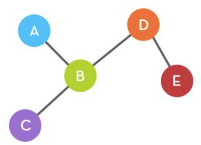
We have said that each node will have an equal probability of being
selected, and that this probability is equal to . Thus each node has a chance of being 39 selected.
An incoming node would choose indiscriminately between the five nodes. So, an incoming node
makes a connection decision with these odds:

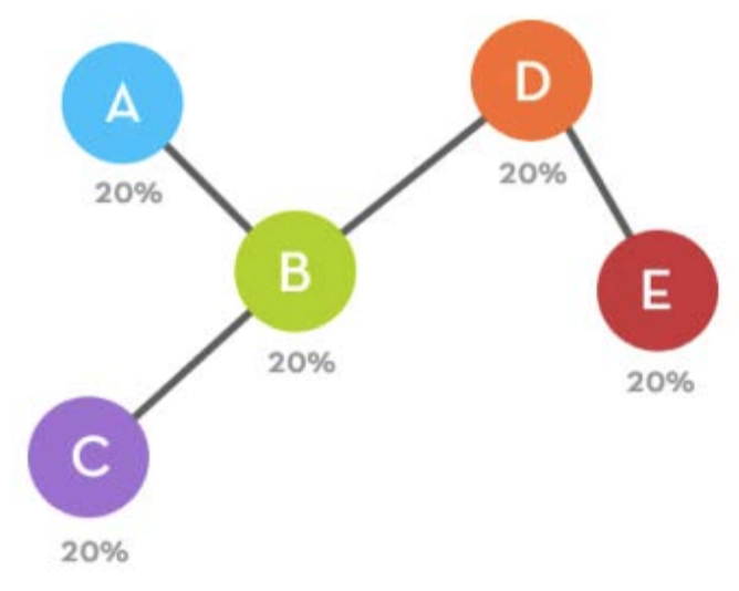
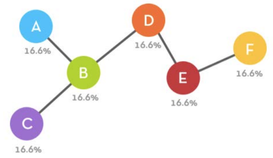
Let’s say that node connects to node . What happens in the next step? Well
now N=6, so each probability is thus. If we were to add a new node, the would follow these
probabilities:

More ERRG

What is considered classical network theory is centered around the
Erdos-Renyi Random Graph (ERRG) model. For our purposes, we will say that a slightly modified ERRG
model adds a new agent to the network with equal probability to all agents. Thus, in a
2-agent networks, nodes A and B can be chosen with equal probability, or its 50% likely that either
will be selected. We can simply model this by flipping a coin: if it’s heads we add a link to a.A,
if it’s tails, we add it to a.B. coin flip outcome: tails Okay, so we flipped a coin and it’s tails, so let’s add it to a.B and
create our second edge, e.2. Now our network looks like this:

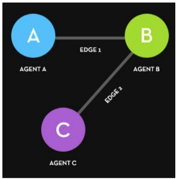
So we’ve added a.C, and now we want to add another node. The question is,
now which one do we pick? This outcome of this decision is ultimately the divergence between
classical and complex network theory. In classical network theory, we would seem to
follow the same process, except this time we have three nodeas and therefore have a 1/3rd
or 33% probability of selecting each node:

If do this process over and over again, we obtain an Erdos-Renyi Random
Graph, where the average node has the average number of links. No node has too many links,
none too few. The degree distribution of a random graph looks like this:

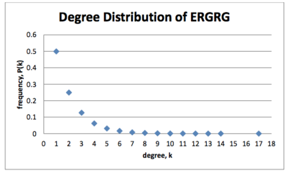
What does this say? Well the x-axis is the number of degrees. The y-axis is
the frequency of this degree occurring. So to interpret this, we would say that 50% of the
nodes have 1 link, about 25% have two links, 12.5% have three links. And his decays
exponentially relatively quickly. Then at the right side of the x-axis we have the more connected
links, which have really low probabilities. For example only 1 node has 17 links, the maximum. This
node occurs 0.002% of the time. In fact, less than 1% of the nodes have more than 7
links. So even after adding 20,000 nodes– twenty thousand nodes–at random, the highest only
had 17 connections. This is not a graph that screams efficient nontrivial topological
self-organization to anyone. We have in effect created a randomly generated network, one without any
discernable

macrostructure based on a probability p. But random networks have a
significant downfall: they poorly represent ‘real-world’ networks. Because network generation is a
cumulative process, we things don’t just happen randomly. In fact, in this
highly entropic scenario, non-trivial self-organization does not occur. Nothing forms in random networks. This is
precisely because the network growth is dependent upon a distribution of
randomness. We have also seen that small rules at the micro-level can result in
macro-level patterns. We have seen that rewiring or generating a network can result in a greater
emergent network property. So far we have discussed structured and random networks, but the
remainder of this Project will be concerned with those of non-trivial structure. It turns out this method of modeling random networks, one which had been
generally for about 50 years prior could not describe the networks that were being discovered
in the late 90s. The degree distributions of real-world scale-free networks just didn’t look
like that. And further, this mechanism of straight-up random attachment didn’t work; it didn’t fit any
data, not static, not dynamic. This problem became more obvious when the ability to obtain and
analyze humongous data sets began to proliferate and the alleged ubiquity of
scale-free networks came into light. To really explain how networks form in
the real world, we need a less random Mechanism.

BAPA Appendix

So let’s do essentially the same thing, except this time with one caveat.
Instead of choosing a node at random, let’s make the decision based on some property of the node.
We need a way to sort of rank the nodes, to make them not equal. Let’s consider analyzing
them by about the only property we know about them other than that they exist, their degree. When we had five nodes, we said that the probability of connecting to node
F was this:

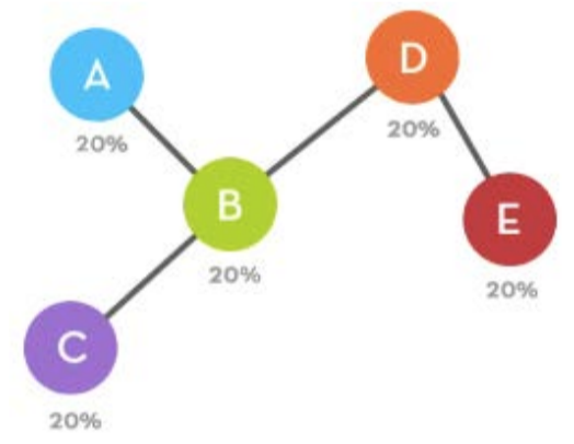
Which means that each node essentially had the odds of being chosen once
every five times in the same way one side of a coin has the odds of being chosen once every two
times:

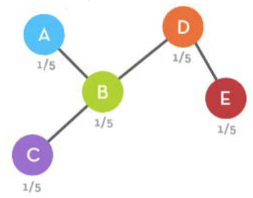
So let’s instead of measuring this probability as 1/N, let’s measure it in
a different way: Ɣ For each node, count up the number of degrees.Ɣ Divide this number by the total number of degrees in the network.
So let’s instead of measuring this probability as 1/N, just picking out any
node at random, we’re weighting it in the sense that we reward those with more degrees. So if we
re-think of the odds, it’s not anymore, because the table is no longer equal:

We see that there are 8 total degrees (because we are only dealing with an
undirected graph so both nodes count one degree to their total, not 1/2 of one), and further we
see that node has the most with 3, next with 2, and the rest with 1. Therefore, the probability
of being chosen as the node is actually 3/8, is 3/8th, and , and are each 1/8th. So what’s the
network emergence implication of this? Let’s look at the graph again, except this time lets
scale it visually to the degree of each node:

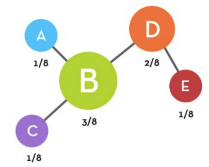
The size is related to the probability that it will be selected. Thus we
immediately see, that B is the most likely to be chosen. In fact, has equal probability as , and of
being chosen combined. This is literally the start of the hub-like evolutionary topology seen in
scale-free networks. Now instead of , this time let’s say the random number generator selected . The
topology is now:

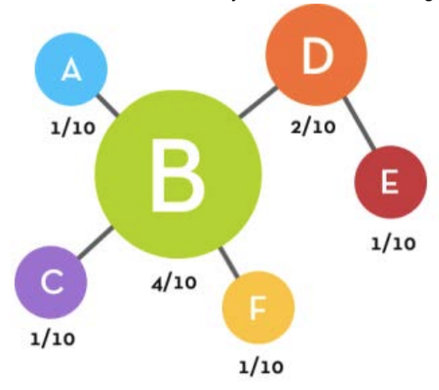
We see that already ‘s positive feedback scheme is already turning the node
into a hub. At each step, this node is more likely to get more and more incoming links. We can
formalize the Barabasi-Albert Preferential Attachment (BAPA) algorithm as:

Ɣ Start with a graph of n nodes,Ɣ At each time-step add m new nodes with probability P(k) = k_i / sum(k_j)
We see that this mechanism does not simply connect at random, and this
biased decision.making is integral to the development of scale-free networks nontrivial
hublike topology. What happens when we run our BAPA mechanism over and over again? What
happens to the degree distribution?

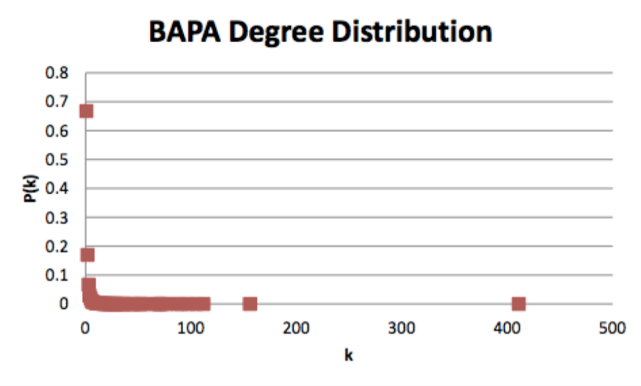
In a way, it almost like it decays like an exponential except for one huge
different. Look at how apparent the hub topology is. The highest node on the ERRG had 17 links.
The highest here, has over 400. The next highest, over 100. Further, there’s a bunch of nodes
of varying degree in between. They’re all very infrequent, but they’re are there and integral to
the integrity of the system.

Let’s put them on the same graph, and discuss the real difference between
these two graphs.

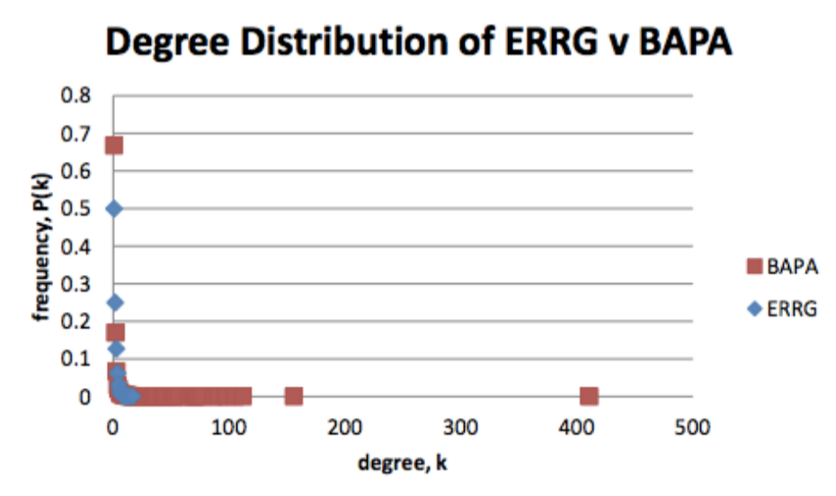
So it’s clear that while the BAPA initially decays at a similar rate with
ERRG, ultimately the exponential decays much faster. The extension of this hub-toplogy, the
right part of the graph where there is red but no blue, this the literally what the ‘long tail’ is
Let’s discuss scale-free network’s claim to fame. If we instead, plot our
data logarithmically, that is on a log-log plot, we see the real nontrivial result of scale-free
networks:

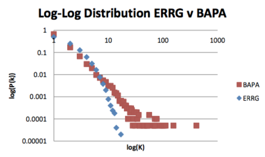
So we see ERRG decays faster, and there are lots of mid-range nodes with
BAPA, but let’s look only over the linear range, which we can do because the hubs — although
they are there — are each an individual case, so their actual position along the x-axis is not
as mandatory to know:

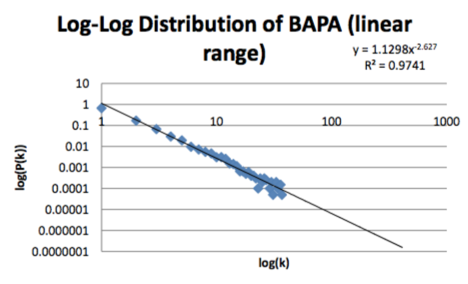
If we project our estimator out with a power-law fit, we see we get a
straight line. And more importantly, we find this line in the network data obtained in the
real-world: in social systems, in technological systems, in biological systems. They all have this line with
an exponent and the exponent, is always such that . Barabasi-Albert Preferential Attachment
therefore makes scale- free networks really well. Preferentiality,If the distribution follows a power law, then we know the generative
mechanism does not result in random attraction. There exists a natural bias toward more connected
nodes, which is preserved with scale-invariance.

We can make a generalization which says that the total number of profile
likes will be related to the future number of profile likes with a probability. That is the current
linear market share of the profile likes is equal to the probability that same percentage of nodes
will connect to that node. However it’s not necessarily true that the value of the profile likes is
static, in the sense that the preferentiality may change over time. It is important to compare the
current rates with one another to understand how the profiles are varying dynamically. Just
because a profile had a signficant number of likes due to their particular place in society, does
not mean they should be benchmarked at this same rate. Socially adept analysts understand that heuristic analysis involves a
variety of perspectives with proper knowledge of each strenghts and limtations.

Show how BAPA measures preferentiality This means that the probability of the market share is related to the
preferentiality or propinquity of additional nodes. This means that we can get an estimate of how the
profile has been behaving recently. This means that the difference Show logarithmic interpretation.